
Introduction
Linear Discriminant Analysis (LDA) is a statistical tool used as a linear classification algorithm. In constrast to logistic regression, it allows multiclass classification. It tries to find the linear combination of attributes which best separate each group, called discriminants. We are using this method for solving the following problem using Python: Wine classification based on chemical composition.
Base Libraries
The following useful python libraries will be needed for plotting and processing data:
import pandas as pd
import matplotlib.pyplot as plt
import seaborn as sns
1. The Dataset
Wine is a common dataset that can be found in the UCI Machine Learning Repository. Let's load it in our Python Notebook:
from ucimlrepo import fetch_ucirepo
wine = fetch_ucirepo(id=109)
X = wine.data.features
y = wine.data.targets

print(wine.variables)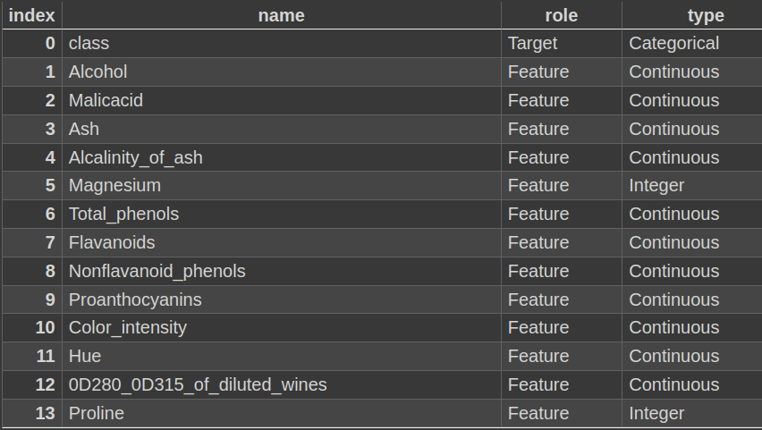
Train and Test Split
To perform a correct testing, let's split 80% of the dataset for training (142 samples), and the remaing 20% for testing (36 samples).
from sklearn.model_selection import train_test_split
X_train, X_test, y_train, y_test = train_test_split(X, y, test_size=0.2, random_state=10)
2. Preparing Data For LDA
To achieve a robust model, we must prepare data to meet the standards expected by the LDA algorithm. In summary, data must:
- Have no missing values
- Have gaussian distributions
- Be standarized
Missing Values
Using the Pandas function X.info() we can confirm that there are no missing values on
the dataset.
Feature Distribution
LDA assumes that each variable have a Gaussian distribution. When examining each one, we can observe that the majority of distributions are correct, although some are skewed.
X_train.hist(layout=(5,5), figsize=(10,10), ec="k", grid=False)
plt.tight_layout()
plt.show()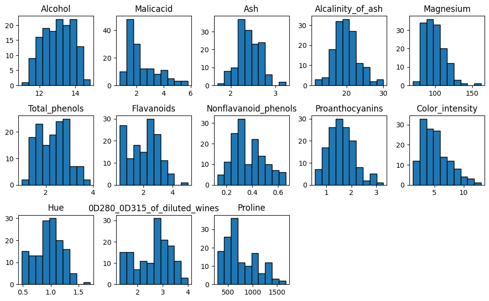
Box-Cox Transformation is a good solution to correct the skewness for each variable, adjusting the Lambda parameter depending on each distribution type. Although, it will not be applyied in this case to simplify the process, but it can be done in the following way:
from scipy.stats import boxcox

color_intensity = X_train['Color_intensity']
corrected_color_intensity = boxcox(color_intensity, lmbda=0.2)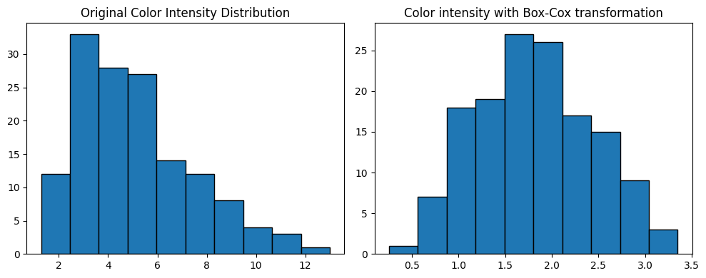
Normalization
Each variable should have the same variance, so we should standarize it to obtain a mean equal to 0, and a standard deviation of 1.
from sklearn.preprocessing import StandardScaler

scaled_data = StandardScaler().fit_transform(X_train)
X_train = pd.DataFrame(scaled_data, columns=X_train.columns)
3. Training LDA model for Classification
It's time to train our classifier with the prepared data. Because LDA is a feature reduction method,
the result will be N - 1 linear discriminant features, where N is the amount of output
classes.
In this case, the result will be 2 discriminants.
from sklearn.discriminant_analysis import LinearDiscriminantAnalysis

lda = LinearDiscriminantAnalysis()
X_lda = lda.fit_transform(X_train, y_train['class'])

plt.figure(figsize=(6, 5))
sns.scatterplot(x=X_lda[:, 0], y=X_lda[:, 1], hue=y_train['class'], palette='Set1')
plt.title('LDA Projection of Data')
plt.xlabel('LDA Discriminant 1')
plt.ylabel('LDA Discriminant 2')
plt.show()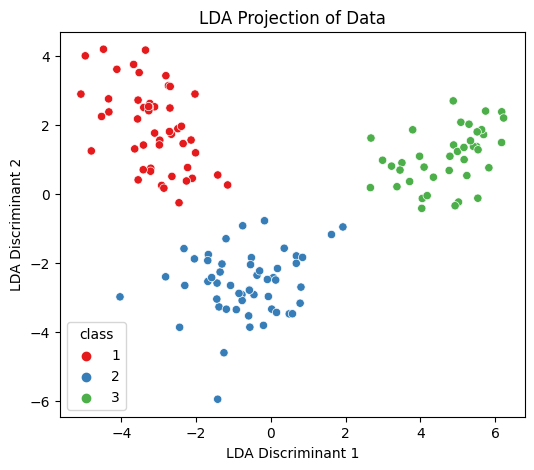
Resulting projection of the data based on the 2 best linear combination of features found (discriminants). There is a clear separation of each cluster of samples.
4. Testing and Performance
Once the classifier is trained, let's make predictions on new data using the remaining test dataset to evaluate its performance.
from sklearn.metrics import classification_report

y_pred = lda.predict(standarize(X_test))
print(classification_report(y_test, y_pred))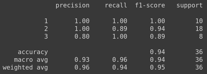
This classification reports show that the model has very good performance on unseen data, with 94% of accuracy.
Confusion Matrix
We can analyze the predictions made with a confusion matrix to compare them with the actual results.
from sklearn.metrics import confusion_matrix

cm = confusion_matrix(y_test, y_pred)
sns.heatmap(cm, annot=True, fmt="d", cmap="Greens", cbar=False,
			xticklabels=y_classes, yticklabels=y_classes)

plt.xlabel('Predicted')
plt.ylabel('Actual')
plt.show()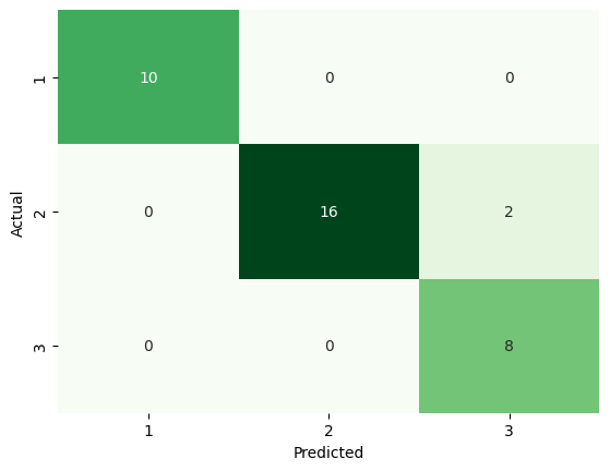
Out of 36 predictions, only 2 mistakes where made. The model classified as Class 3, but was Class 2.
5. Conclusion
The classifier results were really good, achieving a high accuracy of 94% on predictions made for new data. However, the results could be further improved by applying the Box-Cox transformation to each feature with a skewed distribution.
You can find the complete Python Notebook here, which provides more details about the code used.