Car Price Prediction Using Linear Regression

Introduction

Linear Regression is a statistical technique that models the relationship between a dependent variable and a group of independent variables by finding a linear equation that fits the data. It is commonly used in machine learning for making predictions, aiming to minimize the distance between the predicted and actual values.

In the following example we will be predicting car prices based on it's caracteristics, exploring which features are significant to the price and applying feature selection to obtain the optimal amount of features.

Base Libraries

The following useful python libraries will be needed for plotting and processing data:

import pandas as pd
import seaborn as sns
import matplotlib.pyplot as plt
import numpy as np

1. The Dataset

The car prices dataset can be found in Kaggle. It contains data about the American's cars market and pricing. Let's load the csv file into our Python Notebook:

df = pd.read_csv("CarPrice_Assignment.csv")
print(df.info())

2. Data Preprocessing

The dataset contains no missing values, but there are categorical features that must be encoded properly to be used in the linear regression model.

2.1 Categorical Features

Let's take a look at the possible values of each feature:

cat_features = df.select_dtypes(include=['object'])
print(cat_features.apply(lambda feature: feature.unique()))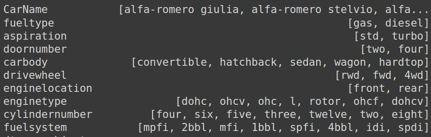

Taking a deeper look to CarName, looks like it's the combination of the brand and model. We will only keep the brand because there are too many models, and probably will not provide much information.

df['brand'] = df.CarName.apply(lambda x: x.split(" ")[0])
df = df.drop(columns=["CarName"])
print("Brands:", np.sort(df.brand.unique()))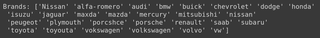

Wait a minute... toyouta?

Unfortunately there are some typos that must be fixed:

df = (df.replace("Nissan", "nissan")
	.replace("vokswagen", "volkswagen").replace("vw", "volkswagen")
	.replace("toyouta", "toyota").replace("maxda", "mazda")
	.replace("porcshce", "porsche").replace("alfa-romero", "alfa-romeo"))

Encoding

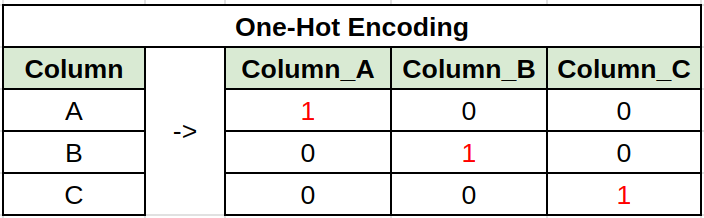
Categorical variables must be encoded to a numerical value for linear regression. For example using label encoding, one-hot encoding, count encoding or many others.
Best results where achieved using label encoding for features with few values, and one-hot encoding for the rest.

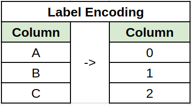
# Label Encoding
label_encoding = ['aspiration','enginelocation','doornumber','fueltype','drivewheel']
df[label_encoding] = df[label_encoding].apply(lambda x: pd.factorize(x)[0])

# One-hot encoding
df = pd.get_dummies(df)

3. Feature Selection

First, let's drop the unrelated feature Car_ID.

df = df.drop(columns=["car_ID"])

Next, we will use a simple but useful approach for feature selection, taking the top best features based on their correlation with the target variable. We can obtain the top and worst 10 features with the following code:

X = df.drop(columns=['price'])
y = df.price
X_by_corr = X.corrwith(y).abs().sort_values(ascending=False)

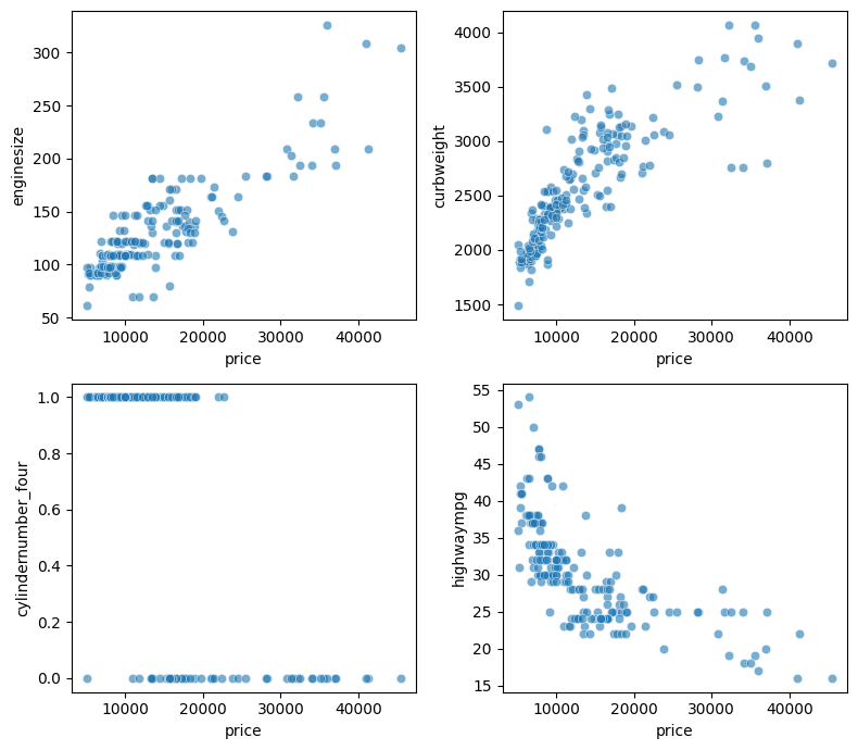
The correlation can be better visualized in scatter plots. For instance, with the following graphs we can conclude that:

• The vehicle's curb weight and engine size directly affects the price
• Cars with four cylinders have low prices
• Higher MPG (Miles Per Gallon) means lower prices

3.1 Finding optimal number of features

To identify the top best features, we will apply cross-validation with 10 folds, using the N most highly correlated variables as the training set for a Linear Regression model. Starting only with the best feature and subsequently incorporating the next best from the list until we have included all of them.
We will use R² and Root Mean Squared Error (RMSE) to evaluate the model performance.

from sklearn.linear_model import LinearRegression
from sklearn.model_selection import cross_validate, KFold

def apply_cross_validation(X, y, kfolds=10):
  model = LinearRegression()
  kf = KFold(n_splits=kfolds, shuffle=True, random_state=42)
  scores = ['r2', 'neg_root_mean_squared_error']
  results = cross_validate(model, X, y, cv=kf, scoring=scores)
  return np.mean(results['test_r2']), -np.mean(results['test_neg_root_mean_squared_error'])

results = {"i": [], "rmse":[], "r2":[]}
for i in range(2, len(X_by_corr)):
  new_X = X[X_by_corr.index[:i]]
  r2, rmse = apply_cross_validation(new_X, y)
  results["i"].append(i)
  results["rmse"].append(rmse)
  results["r2"].append(r2)

results = pd.DataFrame(results)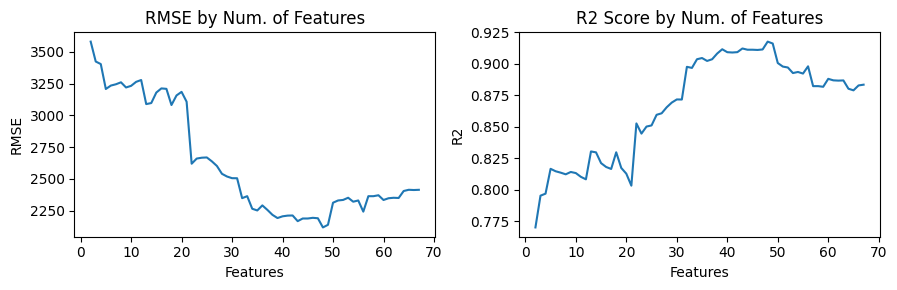

As a result, the optimal number of features is the top 48, with R2=0.918 and RMSE=2118.16. This a good result, so let's filter our final training set:

best = results[results.rmse == results.rmse.min()]
X = X[X_by_corr.index[:best.i.iloc[0]]]

4. Train and Test

Finally, we will split our dataset 80% for training (164 examples) and 20% for testing (41 examples).

from sklearn.model_selection import train_test_split

X_train, X_test, y_train, y_test = train_test_split(X, y, test_size=0.2, random_state=42)

Then, train a Linear Regression model and obtain it's resulting scores.

from sklearn.metrics import r2_score, mean_squared_error
# Train
model = LinearRegression()
model.fit(X_train, y_train)

# Test
y_pred = model.predict(X_test)
rmse = np.sqrt(mean_squared_error(y_test, y_pred))
r2 = r2_score(y_test, y_pred)
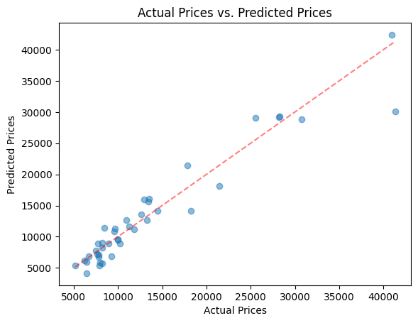
print(f"Test result: RMSE={rmse:.2f}, R2_Score={r2:.3f}")

As a result, the model achieved R2=0.920 and RMSE=2515.90. This means that it had a good performance and accurate predictions, although it could be better.

You can find the complete Python Notebook here, which provides more details about the code used. Remember to download the dataset csv file from Kaggle.